Press enter on a prompt and it can feel like the model understood you, thought it over, and replied. What it actually did is stranger and far simpler. A large language model has one trick: given the text so far, it guesses the next token. Then it adds that token to the text and guesses again. Every billion parameters exists to make that one guess good.
Almost all modern models share the same shape under the hood: a stack of transformer blocks, repeated. Learn the machinery once and you can read most model cards and papers and know which part each section is talking about. So let us follow one sentence the whole way through.
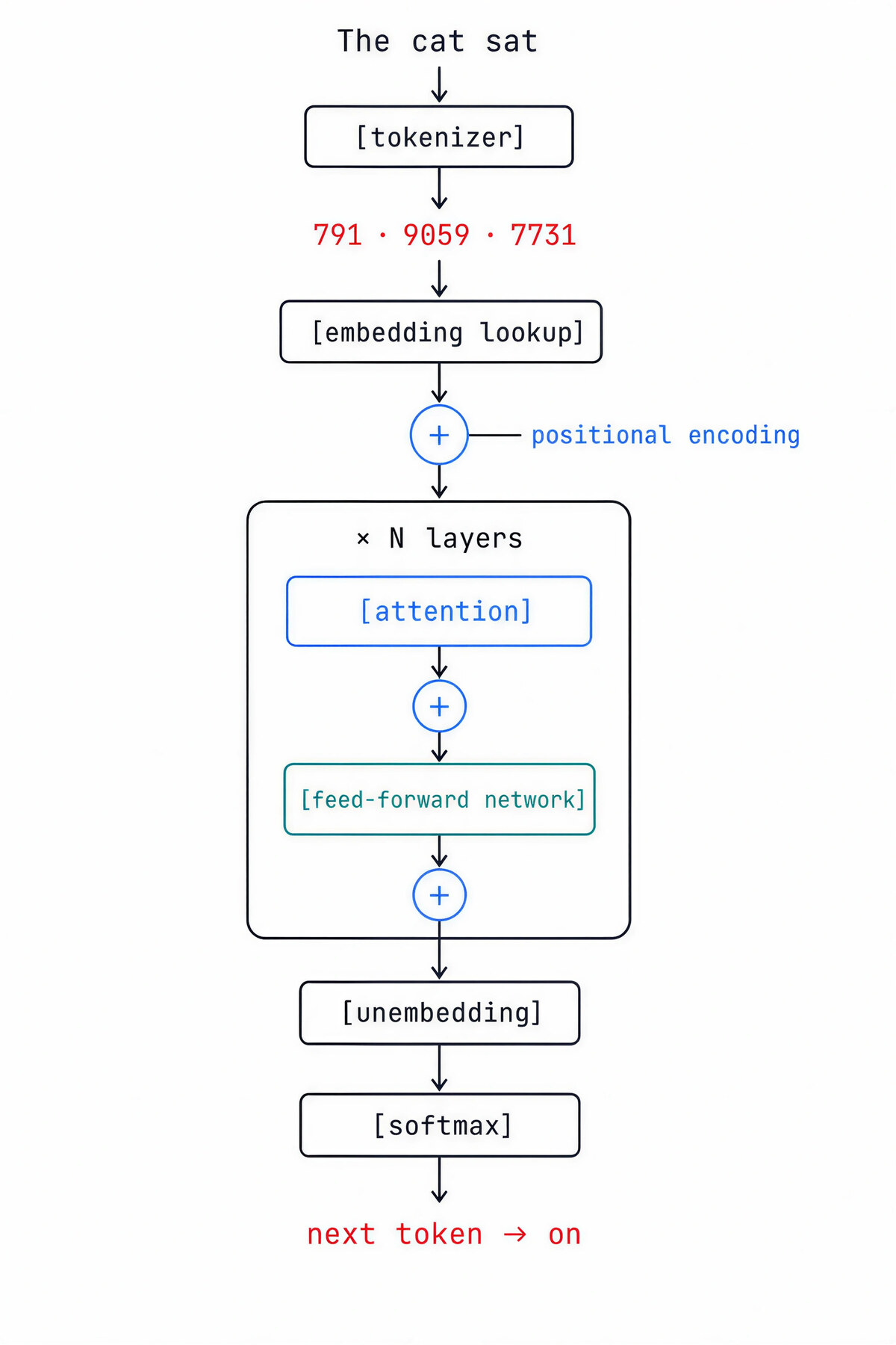
Nine stages. Each one cleans up a problem the previous stage left behind. Here we go.
1. Tokens: text has to become numbers
That something is the tokenizer. It chops the string into pieces and replaces each piece with an integer that points to a row in a fixed list called the vocabulary. Modern vocabularies hold tens of thousands to a few hundred thousand pieces.
The pieces are usually not whole words, they are subword fragments. “tokenization” might become [“token”, “ization”]; “running” might become [“run”, “ning”]. Whole-word vocabularies would be enormous and still miss new words. Letter-by-letter vocabularies would be tiny but force the model to learn everything from scratch. Subwords sit in the middle: common chunks get their own token, rare words are assembled from smaller ones.
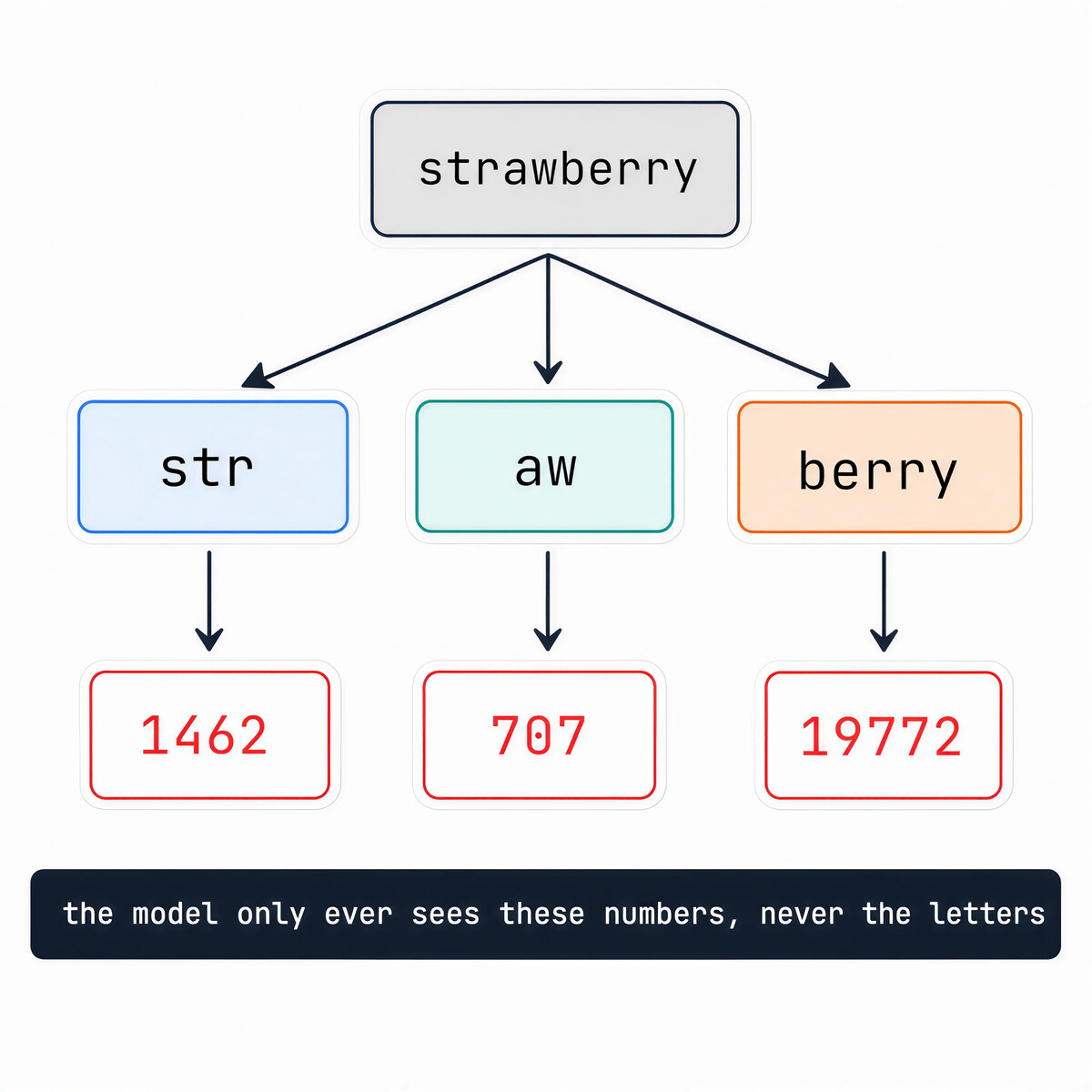
This is why the famous “how many R’s in strawberry” trick stumped models for years. The model never sees s-t-r-a-w-b-e-r-r-y. It sees a couple of token IDs that happen to spell the word to a human. Counting letters it cannot see is hard. Reasoning models do better now, mostly by spelling the word out token by token first, but the root cause was always tokenization, not arithmetic.
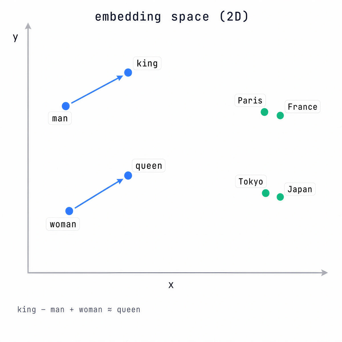
2. Embeddings: numbers have to carry meaning
Meaning comes from the embedding matrix: a giant lookup table with one row per vocabulary entry, where each row is a long list of numbers (a vector). In a 7B-class model that row is often around 4,096 numbers wide. The tokenizer hands over an ID, the model grabs that row, and from now on the token is that vector.
The striking part is what training does to this table on its own. Tokens with similar meanings end up with nearby vectors. “king” lands near “queen,” “Paris” near “France.” Nobody coded that. It falls out of learning to predict text well. You can even do clumsy arithmetic in the space: king minus man plus woman lands close to queen.
One catch. At this stage “dog” has the same vector whether it is the first word of your prompt or the fifth. The meaning is there, the position is not. That is the next problem.
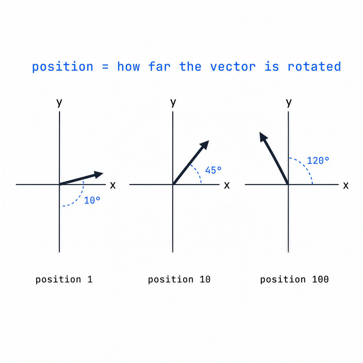
3. Position: order has to be injected
The 2017 transformer fixed this by adding a position pattern to each token’s vector, built from sine and cosine waves so position 1 looked different from position 5. It worked, but it forced one set of numbers to carry both meaning and place, and learned position tables did not stretch past the lengths seen in training.
Most models now use Rotary Position Embeddings (RoPE). Instead of adding a position vector, RoPE rotates each token’s vector by an angle that grows with its position. When two tokens are later compared in attention, what matters is the difference between their rotations, which is exactly the relative distance between them.
Even with good position handling, long prompts show a documented “lost in the middle” effect: models lean on the start and end of a long context more than the middle. That is why “put the important thing first, repeat it at the end” is real advice, not superstition.
4. Attention: tokens have to share information
Attention is the mechanism that gave the architecture its name. Inside every block, each token looks at the other tokens it is allowed to see and decides which ones matter. It does this by casting each token into three roles, three learned vectors: a Query, a Key, and a Value.
A token’s Query is compared against every Key it can see using a scaled dot product, which scores how well two vectors line up. Softmax turns those scores into weights that sum to 1, and the output is a weighted average of the matching Value vectors. High match, high weight, big contribution.
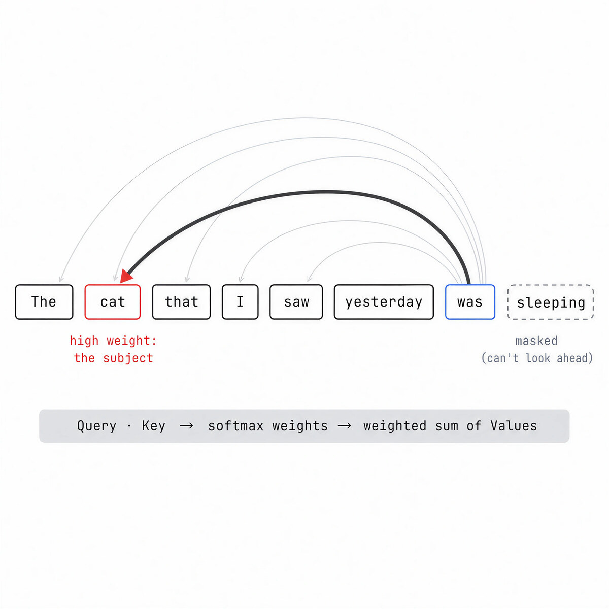
In a left-to-right model there is a rule: a token may only attend to itself and the tokens before it. Future positions are masked, given weights so low they vanish after softmax. That is what keeps the model honest while it predicts the next word.
One of the cleanest findings in interpretability is the induction head: an attention head that spots a pattern like “A B … A” and predicts B again. It is a big part of how a model picks up a pattern from your prompt and continues it, the thing we loosely call in-context learning.
5. Multi-head attention: one view is not enough
So the model runs attention many times in parallel. Each pass is a head with its own learned projections. A point most tutorials get wrong: a head does not get a fixed slice of the token vector. It learns its own small projection of the full vector. With 4,096 numbers and 32 heads, each head works in its own roughly 128-wide space. A different view of the same token, not a different chunk of it.
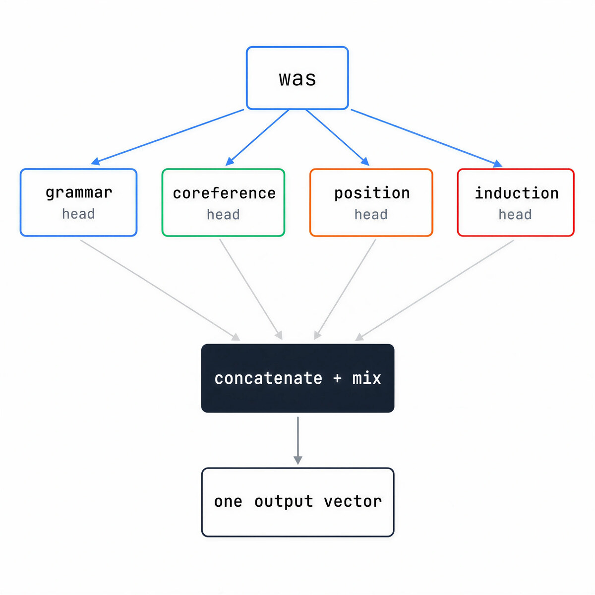
Nobody assigns jobs to heads, the specialization emerges. Researchers have found heads that track grammar, heads that resolve which name a pronoun points to, heads that follow position, induction heads, and many more. A layer might have 32 heads; a frontier model has dozens of layers; so a model carries thousands of heads, each adding its own learned view.
That memory cost drove a real change. In Grouped-Query Attention (GQA) many query heads share a smaller set of key/value heads (LLaMA-2 70B uses 64 query heads but 8 key/value heads). DeepSeek pushed further with Multi-head Latent Attention, which compresses the key/value cache into a small latent vector per token. Similar quality, far less memory, which is a big reason it serves so cheaply.
6. The feed-forward network: each token thinks on its own
That is the feed-forward network, the quieter half of every block. It runs on each token independently, with no cross-token mixing, and does three things: expand the vector to a larger width, apply a non-linearity, then compress it back.
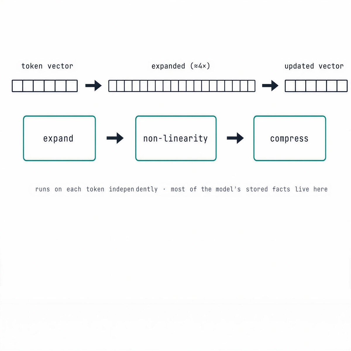
Most of a dense model’s parameters live here, not in attention, and they are not generic. This is where much of the model’s stored knowledge sits. Researchers have found single neurons that fire on a specific concept, and methods like ROME can edit a fact, moving the Eiffel Tower from Paris to Rome, by a targeted tweak to one feed-forward weight matrix, with no retraining.
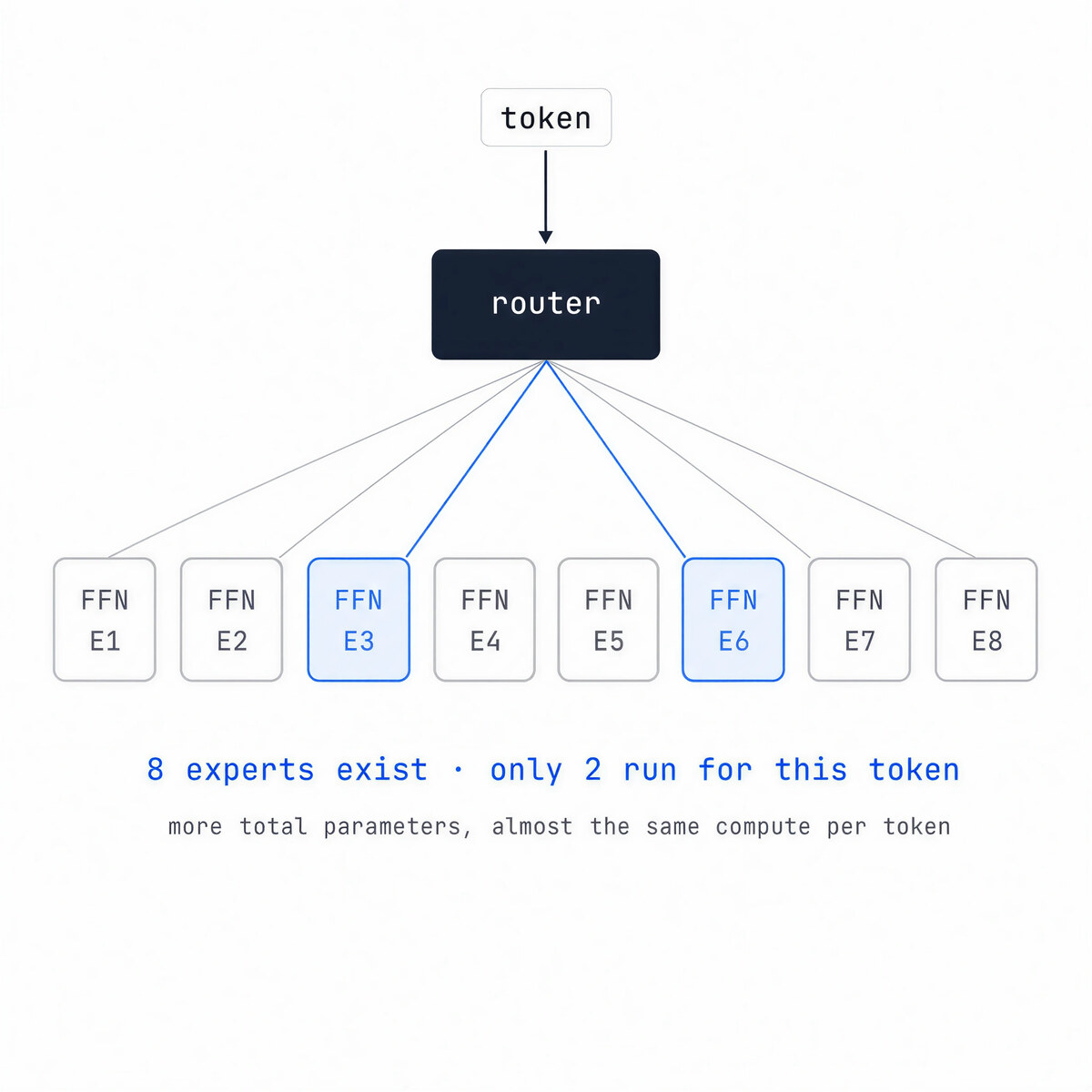
The largest models now often replace one feed-forward network with many. A Mixture of Experts layer holds a set of expert networks plus a tiny router that sends each token to only a couple of them.
7. The residual stream: how a deep stack stays trainable
The first fix is the residual connection. A block’s output is added to its input rather than replacing it. Across the stack this becomes a running sum, the residual stream, with a direct additive path from the input embedding all the way to the end. The trick predates transformers; it came from ResNet in 2015 and made hundred-layer image networks trainable for the first time.
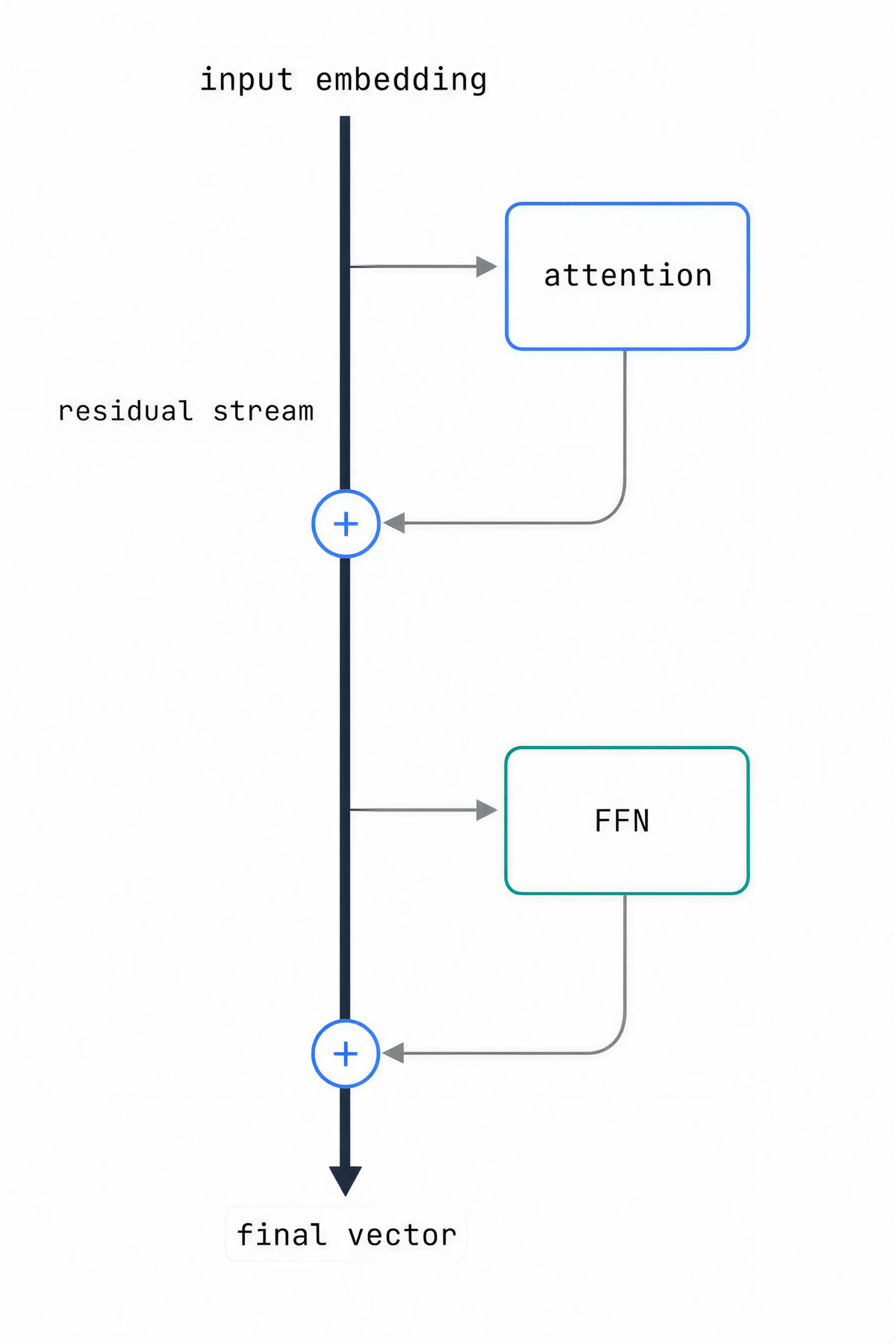
The second fix is normalization, which rescales each token’s vector back into a stable range between sub-blocks so the running sum neither explodes nor vanishes. Two refinements stuck: applying it before each sub-block instead of after (pre-norm), and a cheaper variant called RMSNorm that keeps only the rescaling and drops the mean-centering.
8. Predicting the next token: the loop that writes
After the last block, every token has a final vector. To generate, the model takes the final vector of the last token, and an unembedding step turns it into one raw score per vocabulary entry. With a 100,000-token vocabulary that is 100,000 numbers, called logits.
Softmax turns the logits into a probability distribution, and the model samples from it. It usually does not just take the top choice. Decoding settings shape the output: temperature sharpens or flattens the distribution, top-k and top-p trim it to the plausible candidates. Same model, precise in one setting and playful in another.
Then the chosen token is appended and the whole thing runs again on the longer sequence, reusing the KV cache so the prefix is not recomputed. New vector, new logits, new token. A paragraph is just this loop, one token at a time, until an end token or a length limit. A neat speedup, speculative decoding, lets a small fast model draft several tokens while the big model verifies them in parallel, accepting the run when it agrees. Done right the output matches the big model exactly, but faster.
Everything human-feeling about a chatbot is added afterward, in post-training: instruction tuning, learning from human preferences, safety. The biggest shift of the last two years lives here too. Reasoning models like OpenAI’s o-series and DeepSeek R1 are taught, with reinforcement learning and special “thinking” tokens, to spend more compute at inference, writing a long internal chain of thought before answering. The architecture barely changes. The model simply learns that thinking longer produces better next tokens.
So what is actually different between GPT, Claude, Gemini, and the open models?
Less than the branding suggests, at this level. They sit in the same design space: tokenize, embed, add position, stack blocks of multi-head attention and feed-forward, carry a residual stream, normalize, predict the next token. What varies is three things:
- The trained weights. Different data, different scale, different quality. This is most of the difference you actually feel.
- The configuration. Layer count, vocabulary size, head count, parameter count, dense or Mixture of Experts.
- The post-training. Instruction tuning, preference learning, safety, and now reasoning, all applied on top of the base model.
The interesting thing is how much the field converged. Independent teams arrived at nearly the same modern stack: pre-norm placement, RMSNorm, RoPE, SwiGLU, grouped or latent attention, and Mixture of Experts in the largest models. None of it arrived at once. It accumulated over about five years on top of the 2017 design.
Will it last? Maybe not forever. State-space models like Mamba offer linear-time sequence handling, attractive for very long inputs, and hybrids like Jamba interleave a few attention layers among many state-space layers (plus Mixture of Experts) to hold long contexts cheaply. So far the read is that hybrids win on long, memory-bound serving while attention still wins on associative recall and in-context learning. The safe bet is that the core problems in this post, turning text into numbers, giving numbers meaning and order, letting tokens share information, processing each one, keeping a deep stack trainable, and predicting the next token, outlive whatever architecture is fashionable.
At Kensink Labs we build on top of these models for a living, and the teams that ship reliable AI tend to be the ones who understand the machine they are renting, not the ones chasing the largest number on a leaderboard. Knowing where facts live, why context windows behave oddly, and what post-training can and cannot fix is what separates a demo from a product.
Sources and further reading
- Vaswani et al., Attention Is All You Need (2017). The original transformer.
- Su et al., RoFormer / RoPE (2021). Rotary position embeddings.
- Liu et al., Lost in the Middle (2023). Long-context position bias.
- Olsson et al. (Anthropic), In-context Learning and Induction Heads (2022).
- Meng et al., ROME: Locating and Editing Factual Associations (2022).
- DeepSeek-AI, DeepSeek-V3 Technical Report (2024). MLA and large-scale Mixture of Experts.
- Lieber et al., Jamba: A Hybrid Transformer-Mamba Model (2024).
- Sebastian Raschka, The Big LLM Architecture Comparison (2025).